SensorgramFrom bound mass to a binding curve

A sensorgram records the binding response over time. Here, the response is coherent mass density (CMD). Learn how to interpret association and dissociation, compare optical readouts, and decide whether data support a kinetic model.

Objective. See how coherent mass density over time becomes a binding curve. In the training: One mologram converts patterned binding into one sensorgram.

Recommended first: detection and noise and coherent mass density.

Coherent mass density over time

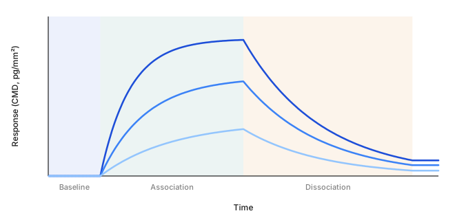
A typical experiment begins with buffer flowing over the surface to establish a baseline. Analyte injection starts the association phase. Switching back to analyte-free buffer starts the dissociation phase. In the ideal model below, the response rises during association and falls during dissociation. Actual traces can differ because of binding behavior, optical bias, or experimental disturbances.

A sensorgram: a flat baseline, a rising association phase during injection, and a falling dissociation phase after switching back to buffer. — Illustrative 1:1 model, not measured data. Three analyte concentrations over the same ligand: higher concentrations associate faster and reach higher. In a simple 1:1 interaction all curves share the same intrinsic dissociation rate.

Read CMD and MD together

CMD reports coherent mass density from the diffracted signal. MD is the refractometric mass-density readout derived from focal-spot position. Bulk index changes can appear as apparent mass in MD.

Illustrative response patterns, not measured traces or unique diagnoses
Observed pattern	Possible explanation	Useful check
MD steps at injection; little CMD change	Sample arrival changes bulk refractive index without much patterned binding.	Inject the same matrix without analyte.
CMD rises after injection; MD may also change	Preferential accumulation on the patterned regions.	Compare non-binding controls and a concentration series.
MD drifts; CMD remains comparatively stable	A common optical disturbance is partly rejected.	Check temperature, buffer stability, and blanks; biological rates may still change.
CMD responds to an analyte-free matrix	Imperfect matching or another optical disturbance contributes to the response.	Inspect blank reproducibility, surface chemistry, and optical alignment.

These patterns narrow the possibilities; they do not identify the bound molecule. A flat CMD trace also cannot prove that no material adsorbed.

What can imitate binding. Ridge-preferential non-specific adsorption; a bulk refractive-index step, which also moves MD; bubbles or fouling that disturb the illumination; an initial optical field of opposite phase, which can make added mass lower the intensity; and a zero crossing, after which the trace runs mirrored. Controls and a relevant blank separate these from target binding.

Frutiger et al. (2021), Part II, Figures 1 to 3 compare the two readouts during binding and refractive-index changes.

What happens to a trace before a fit

The software applies a short chain of cleanup steps before fitting. Each removes one named disturbance.

Blank-mologram subtraction: subtracts what a non-binding mologram saw during the same injections. It removes injection effects and patterned interference that both surfaces share.
Blank-injection subtraction: subtracts a buffer-only injection. It removes what the act of injecting does to the trace.
Normalization to immobilization level: divides each mologram's response by how much ligand it captured, so molograms with different capture become comparable and the fitted maximum response is dimensionless.
Offset removal and trimming: zeroes the trace on the baseline before association and keeps baseline, association and dissociation. A multi-cycle series is first split into its cycles.

None of these steps can add a dissociation phase that was too short or supply missing concentrations. Those are design decisions for a new measurement.

What the shape tells you

For an ideal 1:1 interaction, association depends on analyte concentration and both rate constants. Dissociation without rebinding depends on k_off. The equilibrium dissociation constant is K_D = k_off/k_on. It equals the free analyte concentration at half occupancy under this model. Two interactions can share K_D while having different association and dissociation rates. Interpreting the full curve helps distinguish them.

Two independent estimates of K_D. The kinetic fit gives k_off/k_on. A dose-response fit of the plateau response at each concentration gives K_D as its point of inflection. For well-behaved 1:1 binding the two agree. A Hill slope different from 1 in the dose-response fit means the interaction is not 1:1, and that K_D is an apparent affinity. If the dissociation changes too little to resolve k_off, the result is association rate only: k_on is reported, k_off is below its detection limit, and K_D is unavailable. Only a longer dissociation phase in a new measurement resolves it.

When does a curve support kinetics?

A kinetic fit tests a model against data. A smooth fit alone does not show that its rate constants describe the intended molecular interaction.

Known concentrations: association depends on both concentration and k_on. Unknown active analyte concentration can distort the inferred association rate.
A concentration series: fit multiple concentrations together and inspect residuals. Shared parameters should explain more than one curve.
Controls: matrix blanks and non-binding surfaces help distinguish target binding from injection effects and patterned interference.
Mass transport: analyte delivery can limit association. Where possible, compare flow conditions and ligand densities.
Rebinding: a released molecule can bind again before escaping, slowing the apparent dissociation. Lower surface density can help test this possibility.
Heterogeneous or multivalent binding: mixed sites and avidity can violate a 1:1 model. Do not assign every curved trace a single intrinsic affinity.

For an ideal 1:1 interaction, the observed rate k_obs = k_onc + k_off during association. During dissociation without rebinding, response decays as exp(−k_offt).

Failure of these relationships is a reason to investigate the model and experiment. It is not a reason to add fitting parameters automatically.

For general surface-binding model assumptions, see the Cytiva kinetics handbook, Chapter 12. Its instrument-specific procedures do not apply to the MACS® Matchmaker.

The training covers planning and controls. Reichmuth et al. (2021) provides an assay example with low-affinity binders in complex samples.

Plan the experiment

The training covers experiment planning, controls, and sensorgram interpretation. The MACS Matchmaker documentation covers instrument operation.

Take the training →

Predict before revealing the explanation. Can the single streptavidin association trace establish both rate constants and affinity?

Reveal the explanation

Not by itself. This panel lacks a dissociation phase and a concentration series. Binding stoichiometry and model suitability also need justification.

Takeaway. With known analyte concentrations and a justified binding model, fitting sensorgrams can estimate k_on, k_off and K_D. Shape alone does not establish those values.

Previous
← Detection and noise Next
Glossary and papers →